Introduction
The pdppy package consists of four modules:
- Instances handles input graphical instances for solving,
- Algorithms provides implementations for solving provided PDP instances,
- Plot creates visualizations of instances and their solutions, and
- Helper assists each module in the handling of instances.
The main takeaway from this structure is that the user provides inputs to any one of the functions in the instances.py module.
Then, the outputs from the instances.py module can be fed directly as inputs to any one of the functions in the algorithms.py module.
The outputs from the algorithms.py and instances.py module can then be viewed in conjunction through the plot.py module.
Basics
Learn how to use the pdppy module!
Nodes
Nodes in the graphical instances carry the necessary information for applying any method in algorithms.py. Nodes in a graph can either be a source node s, a target node t, or part of an origin-destination request pair. For this version of the PDP, there can be only one s and one t and as many as k request pairs, each containing an origin (codified as ‘o’) and a destination (codified as ‘d’).
In the instances module, the user may provide values for each of these entries to obtain a desired request graph. The values for s and t can be any singular nodes found in the original input graph. The values for the request_pairs must be a list containing each node pair from the original graph to be treated as a request [(o_1, d_1), …, (o_k, d_k)]; here the ‘request type’ is ‘o’ or ‘d’, and the ‘request number’ is 1 through k for each request pair. If these values are not supplied, a pseudo-random selection of nodes will be chosen from the input graph.
When the request graph is output by the instances.py module from the user’s input, the node labelling is changed for simplification in the algorithms.py module. The original node labels are preserved in the node attribute ‘original’ of the outputted request graph.
For example, if a node ‘y’ in the original graph G is arbitrarily labelled as 3 in the resulting request graph H, then:
>>> H.node[3]['original']
'y'
As mentioned above, failure by the user to specify the nodes for s, t, and request_pairs from the input graph in the instances.request_graph function will result in a random selection of these nodes from the input graph. The seed used for this random selection will be stored as a graph attribute of the output graph under the name ‘seed’ so that the graph may be reproduced by the user.
For example, if the computer had set the seed to be 123456, then:
>>> H.graph['seed']
123456
Graphs
All PDP instances are represented as graphs and are handled as NetworkX graph objects. The graphs handled in this package fall into one of three classifications.
Input Graph
An input graph G is a user-provided graph for the instances.py module and should meet the following criteria:
- The edges of G are undirected: (u, v) = (v, u) and have associated positive weight
- G is connected (any node is reachable from any other node along the edges of G)
- The edges of G have associated positive weight
Take the following example with user-provided G:
>>> import networkx as nx
>>> G = nx.Graph()
>>> G.add_weighted_edges_from([(1, 3, 1.23), (3, 4, 5),('c', 3, 2), (8, 1, 3.6), (1, 'x', 8), ('x', 'y', 10),(4, 'x', 6.4), ('c', 'x', 4.3)])
>>> list(G.nodes())
[1, 3, 4, 8, 'x', 'y', 'c']
>>> nx.is_directed(G)
False
>>> nx.is_connected(G)
True
>>> G.edges[1,3]
{'weight': 1.23}
Request (PDP) Graph
A request graph H is a modification of the input/generated graph G by the instances.py module.
This graph follows a strict structure in the information it carries for the usage of all the modules and, as
a result, should not be modified after it has been produced by any of the instances.py functions.
H is a NetworkX graph that:
- Satisfies the criteria of the input graph G
- Contains only the user-specified nodes from G that will make up the s, t, and request_pairs nodes
- Is metrically closed (complete) over all its nodes
- Stores the additional graph attributes seen below (accessible through H.graph[‘attribute_name’])
User inputs of s = 3, t = 8, and request_pairs = [(1, 4), (‘x’, ‘y’)] on the above example input graph G produce a request graph H that will be a metric closure on these nodes and have the following nodes and attributes:
>>> list(H.nodes())
[1, 3, 4, 8, 'x', 'y']
>>> H.graph['s']
3
>>> H.graph['t']
8
>>> H.graph['requests']
{3: (0, 's'), 8: (0, 't'), 1: (1, 'o'), 4: (1, 'd'), 'x': (2, 'o'), 'y': (2, 'd')}
Tour Graph
A tour graph P is a graphical representation of the solution produced by one of the methods in the algorithms.py module. It contains all the nodes in the request graph and contains only the edges that appear in the solution. The tour graph P contains two additional graph attributes ‘dist’ for the total tour distance and ‘type’ for the method in algorithms.py used to produce P.
For example, if P had a total tour distance of 5.8 and was computed by algorithms.cheapest_feasible_insertion which has type code ‘CFI’, then:
>>> P.graph['dist']
5.8
>>> P.graph['type']
'CFI'
The edges of P contain an attribute ‘value’ which hold the edge’s value in the solution. The values associated with this attribute should be 1 for every edge from all methods with the exception of the tours produced by the algorithms.linear_prog method which may have fractional values corresponding to the non-integer solution values found by the linear programming solver.
Tutorial
This is a complete example for the use of the different modules and the functions within.
Import the modules, the NetworkX package, and any others you may need.
>>> import pdppy as pdp
>>> import networkx as nx
Supply your own NetworkX input graph G and nodes for selection.
>>> G = nx.Graph()
>>> G.add_weighted_edges_from([(1, 3, 1.23), (3, 4, 5),('c', 3, 2), (8, 1, 3.6), (1, 'x', 8), ('x', 'y', 10),(4, 'x', 6.4), ('c', 'x', 4.3)])
>>> H = pdp.instances.request_graph(G, 3, 8, [(1, 4), ('x', 'y')])
Or, use the instances.random_geo_graph function to generate an input and request graph with 3 request pairs and a seed of 10001.
>>> G2, H2 = pdp.instances.random_geo_graph(3, 10001)
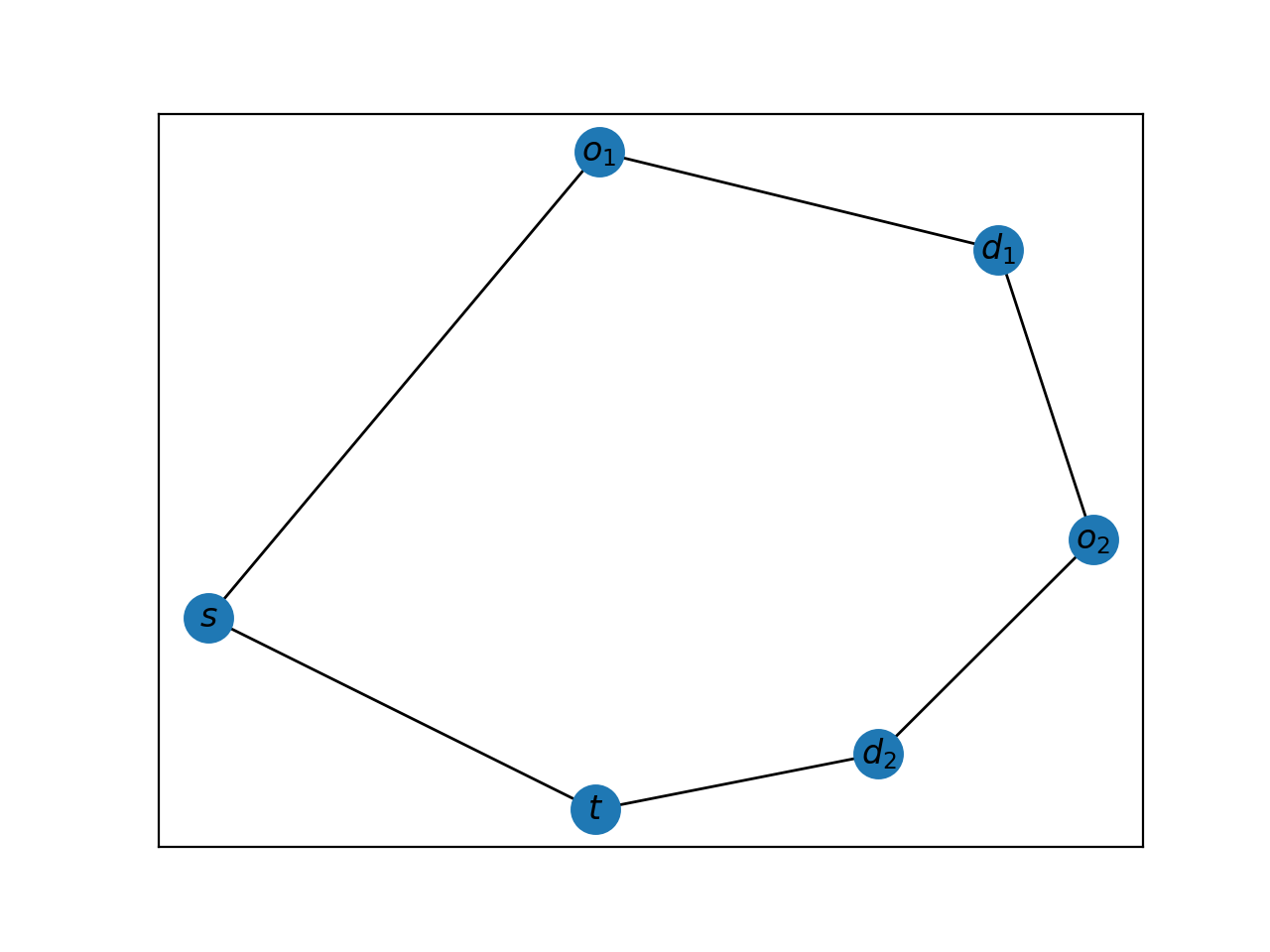
Using the request graph, compute the solution using one of the methods in algorithms.py.
>>> P = pdp.algorithms.path_build_alg(H)
Analyze and visualize the solution using the function plot.plot_tour.
>>> P.graph['dist']
49.82
>>> pdp.plot.plot_tour(P)
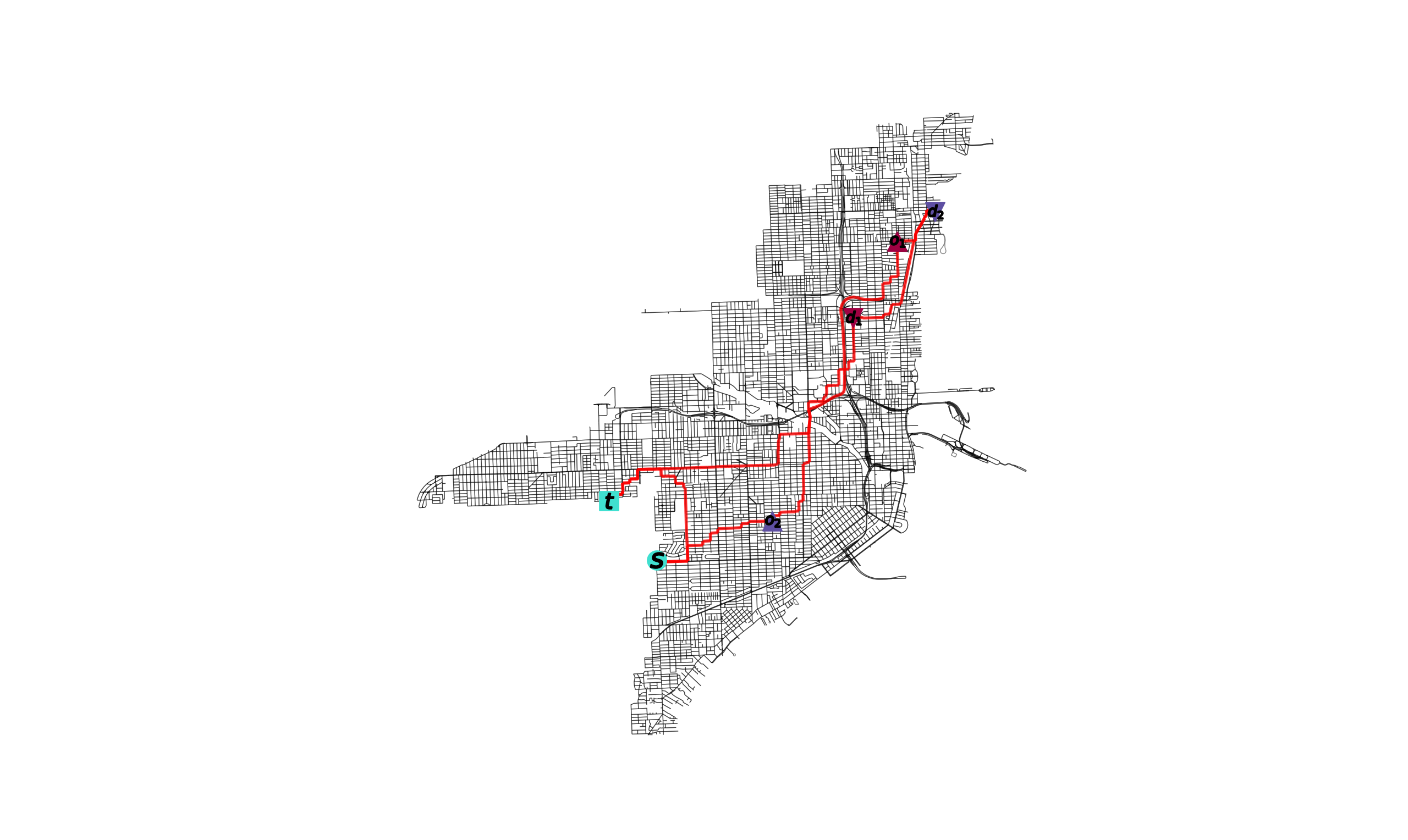
For working with an OSMnx graph, simply use the instances.city_graph function and query the desired city through the city parameter.
>>> import pdppy as pdp
>>> import networkx as nx
>>> G, H = pdp.instances.city_graph('Miami, USA', k=3, seed=10001)
The road network could also be supplied by the user in the case a specific kind of road network is desired by the user.
>>> import osmnx as ox
>>> G = ox.graph_from_place('Miami, USA', network_type='walk')
>>> G, H = pdp.instances.city_graph('Miami, USA', G=G, k=3, seed=10001)
A tour can then be computed over the resulting request graph H using one of the functions in algorithms.py.
>>> P = pdp.algorithms.four_traversal_mst_alg(H)
>>> P.graph['dist']
37243.63
Can overlay tour P on OSMnx graph G.
>>> pdp.plot.plot_tour(P, G)